Discrete outcome regression
quasi_plot() generates QQ-plots for regression models
with discrete outcomes, employing quasi-empirical residual distribution
functions. It’s tailored to assess model assumptions in GLMs featuring
binary, ordinal, Poisson, negative binomial, zero-inflated Poisson, and
zero-inflated negative binomial outcomes. Unlike typical functions in
assessor package, quasi_plot() exclusively
focuses on plotting QQ-plots and does not compute DPIT residuals.
- Negative binomial,
MASS::glm.nb() - Poisson,
glm(formula, family=poisson(link="log")) - Binary,
glm(formula, family=binomial(link="logit")) - Ordinal,
MASS::polr() - Zero-Inflated Poisson,
pscl::zeroinfl(dist = "poisson") - Zero-Inflated negative binomial,
pscl::zeroinfl(dist = "negbin")
The tabs below explain how to interpret the QQ-plots generated by
quasi_plot() in Poisson and Zero-inflated Poisson examples,
respectively.
We simulate a Poisson random variable using covariates and . The true mean of is intricately connected to both and , as expressed in the ensuing relationship: where .
library(assessor)
## Poisson example
n <- 500
set.seed(1234)
# Covariates
x1 <- rnorm(n)
x2 <- rbinom(n, 1, 0.7)

# Coefficients
beta0 <- -2
beta1 <- 2
beta2 <- 1
lambda1 <- exp(beta0 + beta1 * x1 + beta2 * x2)
y <- rpois(n, lambda1)
# True model
poismodel1 <- glm(y ~ x1 + x2, family = poisson(link = "log"))
quasi_plot(poismodel1)
#> Multistart 1 of 1 |Multistart 1 of 1 |Multistart 1 of 1 |Multistart 1 of 1 /Multistart 1 of 1 |Multistart 1 of 1 | 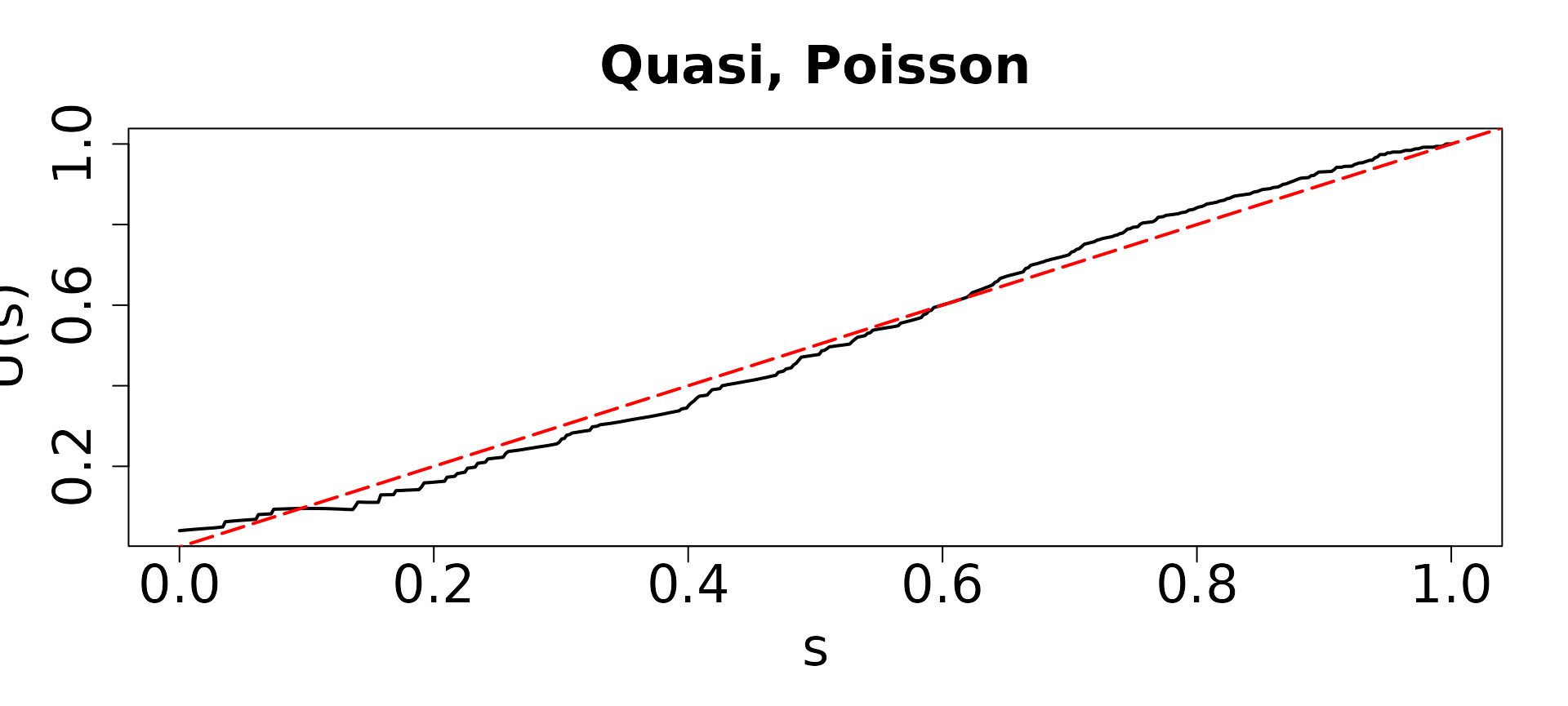 The figure presented above represents the results of
poismodel1, which is a GLM fitted with a Poisson
distribution. In this context, the variable y follows a
Poisson distribution as defined in the model. Our expectation was that
the QQ-plot would exhibit alignment with diagonal lines, as this
alignment indicates conformity with the assumptions of the Poisson
distribution for discrete outcome regression.
As anticipated, the result indeed demonstrates a well-aligned QQ plot, closely following the diagonal line. This alignment is indicative of the correctness of our model assumption regarding the distribution of the outcome variable. In simpler terms, it suggests that our model is appropriately capturing the characteristics of the data, specifically the discrete nature of the outcomes, as dictated by the Poisson distribution.
We generate simulated data using a zero-inflated Poisson model. The probability of excess zeros is modeled using , while the Poisson component has a mean of . Here, follows a normal distribution with mean 0 and standard deviation 1, and is a binary variable with a probability of 1 set to 0.7. The parameter values are set to .
## Zero-Inflated Poisson
library(assessor)
library(pscl)
n <- 500
set.seed(1234)
# Covariates
x1 <- rnorm(n)
x2 <- rbinom(n, 1, 0.7)
# Coefficients
beta0 <- 0.5
beta1 <- 2
beta2 <- 1
beta00 <- -2
beta10 <- 2

# Mean of Poisson part
lambda1 <- exp(beta0 + beta1 * x1 + beta2 * x2)
# Excess zero probability
p0 <- 1 / (1 + exp(-(beta00 + beta10 * x1)))
## simulate outcomes
y0 <- rbinom(n, size = 1, prob = 1 - p0)
y1 <- rpois(n, lambda1)
y <- ifelse(y0 == 0, 0, y1)
par(mfrow=c(1,2))
## True model
modelzero1 <- zeroinfl(y ~ x1 + x2 | x1, dist = "poisson", link = "logit")
quasi_plot(modelzero1)
#> Multistart 1 of 1 |Multistart 1 of 1 |Multistart 1 of 1 |Multistart 1 of 1 /Multistart 1 of 1 |Multistart 1 of 1 |
## Zero inflation
modelzero2 <- glm(y ~ x1 + x2, family = poisson(link = "log"))
quasi_plot(modelzero2)
#> Multistart 1 of 1 |Multistart 1 of 1 |Multistart 1 of 1 |Multistart 1 of 1 /Multistart 1 of 1 |Multistart 1 of 1 | 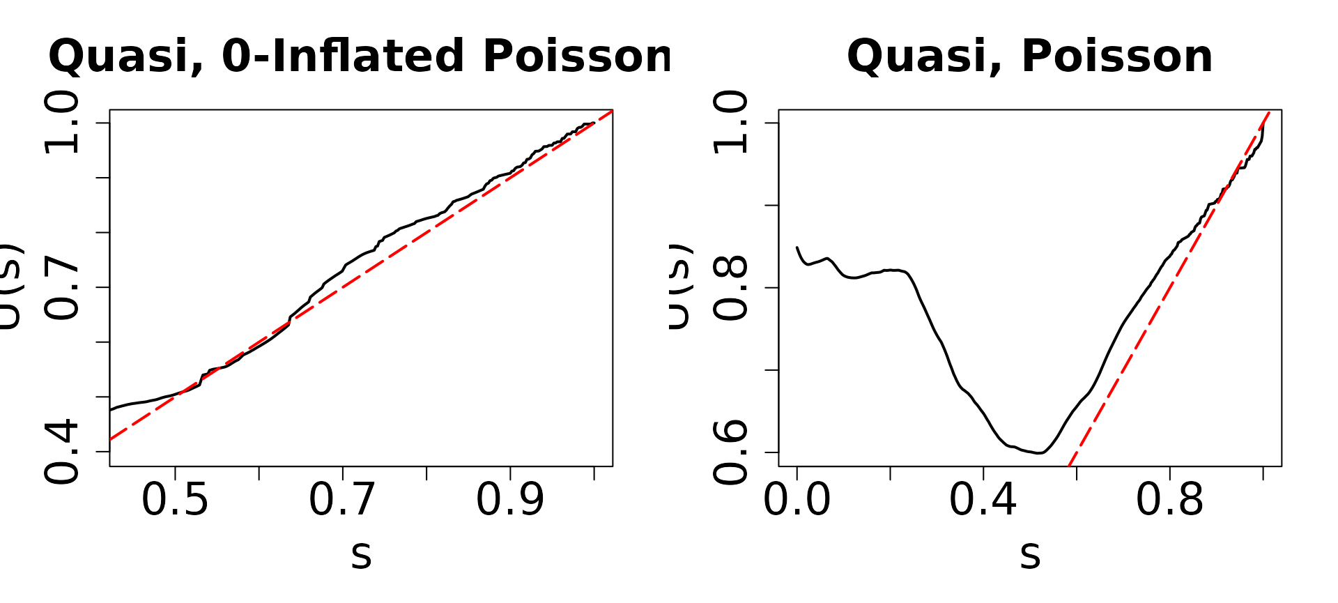 The QQ plots shown above correspond to
 modelzero1 and
modelzero2. Given that the true distribution of
y follows a zero-inflated Poisson distribution, we expect
to see deviations from the diagonal line in the QQ plot of
modelzero2. As anticipated, the QQ plot on the left closely
follows the diagonal line. However, in the right panel, both the left
and right tails of the QQ plot for modelzero2 deviate from
the diagonal line, indicating that the assumption of a Poisson
distribution may not be accurate.
The observed differences in the QQ plot of modelzero2
suggest that the assumption of a Poisson distribution is not
well-supported by the data. This underscores the importance of
considering alternative distributional assumptions, such as the
zero-inflated Poisson distribution, which may better capture the
characteristics of the simulated data.