Discrete outcome regression models
dpit() is used for calculating the DPIT residuals for
regression models with discrete outcomes and constructing their
QQ-plots. The suitable model objects are as follows:
- Negative binomial,
MASS::glm.nb() - Poisson,
glm(formula, family=poisson(link="log")) - Binary,
glm(formula, family=binomial(link="logit")) - Ordinal,
MASS::polr()
An example of the usage of the dpit() function for a
negative binomial regression is included below. The data are generated
using a negative binomial distribution with mean
,
where
,
and
is binary with a probability of success as 0.7. The coefficients are set
as
,
and
.
The underlying size parameter is 2. To assess model assumptions, one can
employ a QQ-plot generated through either reisd_disc() or
qqresid().
library(assessor)
library(MASS)
n <- 500
set.seed(1234)
## Negative Binomial example
# Covariates
x1 <- rnorm(n)
x2 <- rbinom(n, 1, 0.7)

### Parameters
beta0 <- -2
beta1 <- 2
beta2 <- 1
size1 <- 2
lambda1 <- exp(beta0 + beta1 * x1 + beta2 * x2)

# generate outcomes
y <- rnbinom(n, mu = lambda1, size = size1)
par(mfrow=c(1,2))
# True model
model1 <- glm.nb(y ~ x1 + x2)
resd1 <- dpit(model1, plot = TRUE, scale = "normal")

# Overdispersion
model2 <- glm(y ~ x1 + x2, family = poisson(link = "log"))
resd2 <- dpit(model2, plot = TRUE, scale = "normal")
The
The model1 is correctly specified as a GLM with a negative
binomial distribution, whereas model2 incorrectly assumes
the Poisson family, and thus overdispersion is present. The left panel
displays a diagonal QQ-plot along the straight red line, indicative of
the model assumption holding. In contrast, the right panel deviates from
a diagonal line, suggesting a lack of adherence to the assumption. In
addition, in an overdispersed model, due to the underestimated variance,
a S-shaped pattern presents in the QQ-plot.
Similarly, we can simulate a Poisson random variable using covariates and . The true mean of is intricately connected to both and , as expressed in the ensuing relationship: where .
## Poisson example
n <- 500
set.seed(1234)
# Covariates
x1 <- rnorm(n)
x2 <- rbinom(n, 1, 0.7)

# Coefficients
beta0 <- -2
beta1 <- 2
beta2 <- 1
lambda1 <- exp(beta0 + beta1 * x1 + beta2 * x2)
y <- rpois(n, lambda1)
We manually enlarged three outcomes by adding values of 10, 15, and 20 to them, respectively. In the right panel, we can see the three modified data points stand out, signaling they are potential outliers.
par(mfrow=c(1,2))
# True model
poismodel1 <- glm(y ~ x1 + x2, family = poisson(link = "log"))
resid1 <- dpit(poismodel1, plot = TRUE)

# Enlarge three outcomes
y <- rpois(n, lambda1) + c(rep(0, (n - 3)), c(10, 15, 20))
poismodel2 <- glm(y ~ x1 + x2, family = poisson(link = "log"))
resid2 <- dpit(poismodel2, plot = TRUE)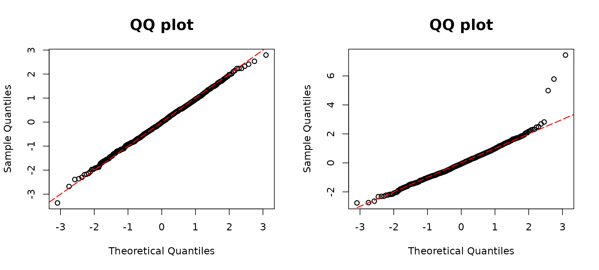
For the binary example, generate Bernoulli random variable, , whose mean depends on covariates and . The underlying model is a logistic regression with the probability of 1 as , where , , and is a dummy variable with a probability of one equal to 0.7.
## Binary example
n <- 500
set.seed(1234)
# Covariates
x1 <- rnorm(n, 1, 1)
x2 <- rbinom(n, 1, 0.7)
# Coefficients
beta0 <- -5
beta1 <- 2
beta2 <- 1
beta3 <- 3
q1 <- 1 / (1 + exp(beta0 + beta1 * x1 + beta2 * x2 + beta3 * x1 * x2))

y1 <- rbinom(n, size = 1, prob = 1 - q1)
For the misspecified model, the binary covariate and the interaction term are omitted.
par(mfrow=c(1,2))
# True model
model01 <- glm(y1 ~ x1 * x2, family = binomial(link = "logit"))
resid1 <- dpit(model01, plot = TRUE)
# Missing covariates
model02 <- glm(y1 ~ x1, family = binomial(link = "logit"))
resid2 <- dpit(model02, plot = TRUE)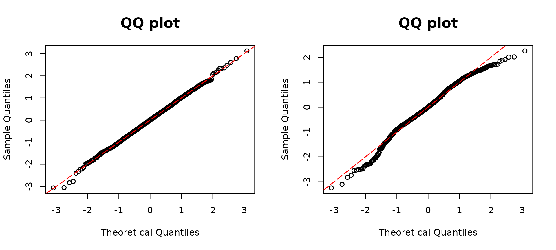 The true model, distinguished as
 model1, is visually
represented in the left panel, showcasing an alignment with the red
diagonal line. This alignment serves as an indicator of the model’s
adherence to the expected pattern. On the other hand,
model2, made without the inclusion of the variable
and the interaction, presents a deviation from the prescribed red
diagonal line.
Our dpit() function is also applicable to ordinal
regression fitted by MASS::polr(). In this experiment, we
consider ordinal regression models with three levels 0, 1, and 2. Under
an ordinal logistic regression model with proportionality assumption,
where
is the distribution function of a logistic random variable with mean
.
We let
,
,
,
and
.
## Ordinal example
n <- 500
set.seed(1234)
# Covariates
x1 <- rnorm(n, mean = 2)
# Coefficient
beta1 <- 3

# True model
p0 <- plogis(1, location = beta1 * x1)
p1 <- plogis(4, location = beta1 * x1) - p0
p2 <- 1 - p0 - p1
genemult <- function(p) {
  rmultinom(1, size = 1, prob = c(p[1], p[2], p[3]))
}
test <- apply(cbind(p0, p1, p2), 1, genemult)
y1 <- rep(0, n)
y1[which(test[1, ] == 1)] <- 0
y1[which(test[2, ] == 1)] <- 1
y1[which(test[3, ] == 1)] <- 2
multimodel <- polr(as.factor(y1) ~ x1, method = "logistic")
We then generate data under the scenario where the assumption of proportionality is not met, which is a common issue for ordinal regression models. Specifically, as described above whereas , where is the distribution function of a logistic random variable with mean and we set . The data are incorrectly fit with a proportional odds model.
## Non-Proportionality
n <- 500
set.seed(1234)
x1 <- rnorm(n, mean = 2)
beta1 <- 3
beta2 <- 1
p0 <- plogis(1, location = beta1 * x1)
p1 <- plogis(4, location = beta2 * x1) - p0
p2 <- 1 - p0 - p1
genemult <- function(p) {
  rmultinom(1, size = 1, prob = c(p[1], p[2], p[3]))
}
test <- apply(cbind(p0, p1, p2), 1, genemult)
y1 <- rep(0, n)
y1[which(test[1, ] == 1)] <- 0
y1[which(test[2, ] == 1)] <- 1
y1[which(test[3, ] == 1)] <- 2
multimodel2 <- polr(as.factor(y1) ~ x1, method = "logistic")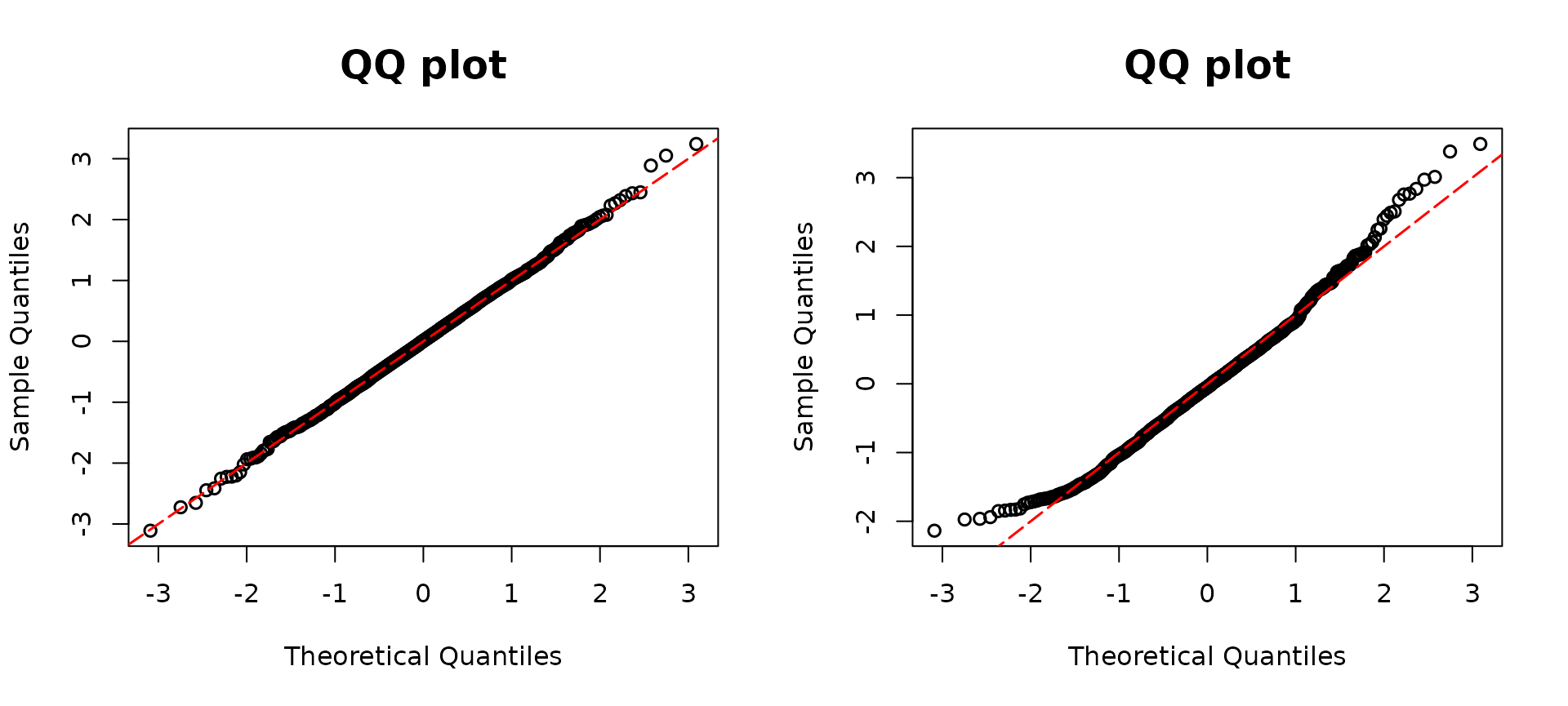 As a result, when considering the diagnostic assessment through
QQ-plots,
As a result, when considering the diagnostic assessment through
QQ-plots, model1 exhibits a diagonal QQ-plot, indicating a
favorable alignment with the underlying assumptions. In contrast, the
QQ-plot associated with model2 deviates from the expected
diagonal line, suggesting a departure from the idealized model
assumptions. This discrepancy underscores the importance of careful
consideration and inclusion of relevant variables in model specification
to ensure the robustness and validity of statistical models.