Residuals for regression models with negative binomial outcomes

Computes DPIT residuals for regression models with negative binomial outcomes using the observed counts (y) and their fitted distributional parameters (mu, size).

Usage

dpit_nb(y, mu, size, plot=TRUE, scale="normal", line_args=list(), ...)

Arguments

y: An observed outcome vector.
mu: A vector of fitted mean values.
size: A dispersion parameter of the negative binomial distribution.
plot: A logical value indicating whether or not to return QQ-plot
scale: You can choose the scale of the residuals among normal and uniform. The sample quantiles of the residuals are plotted against the theoretical quantiles of a standard normal distribution under the normal scale, and against the theoretical quantiles of a uniform (0,1) distribution under the uniform scale. The default scale is normal.
line_args: A named list of graphical parameters passed to graphics::abline() to modify the reference (red) 45° line in the QQ plot. If left empty, a default red dashed line is drawn.
...: Additional graphical arguments passed to stats::qqplot() for customizing the QQ plot (e.g., pch, col, cex, xlab, ylab).

Value

DPIT residuals.

Details

For formulation details on discrete outcomes, see dpit.

Examples

## Negative Binomial example
library(MASS)
n <- 500
x1 <- rnorm(n)
x2 <- rbinom(n, 1, 0.7)
### Parameters
beta0 <- -2
beta1 <- 2
beta2 <- 1
size1 <- 2
lambda1 <- exp(beta0 + beta1 * x1 + beta2 * x2)
# generate outcomes
y <- rnbinom(n, mu = lambda1, size = size1)

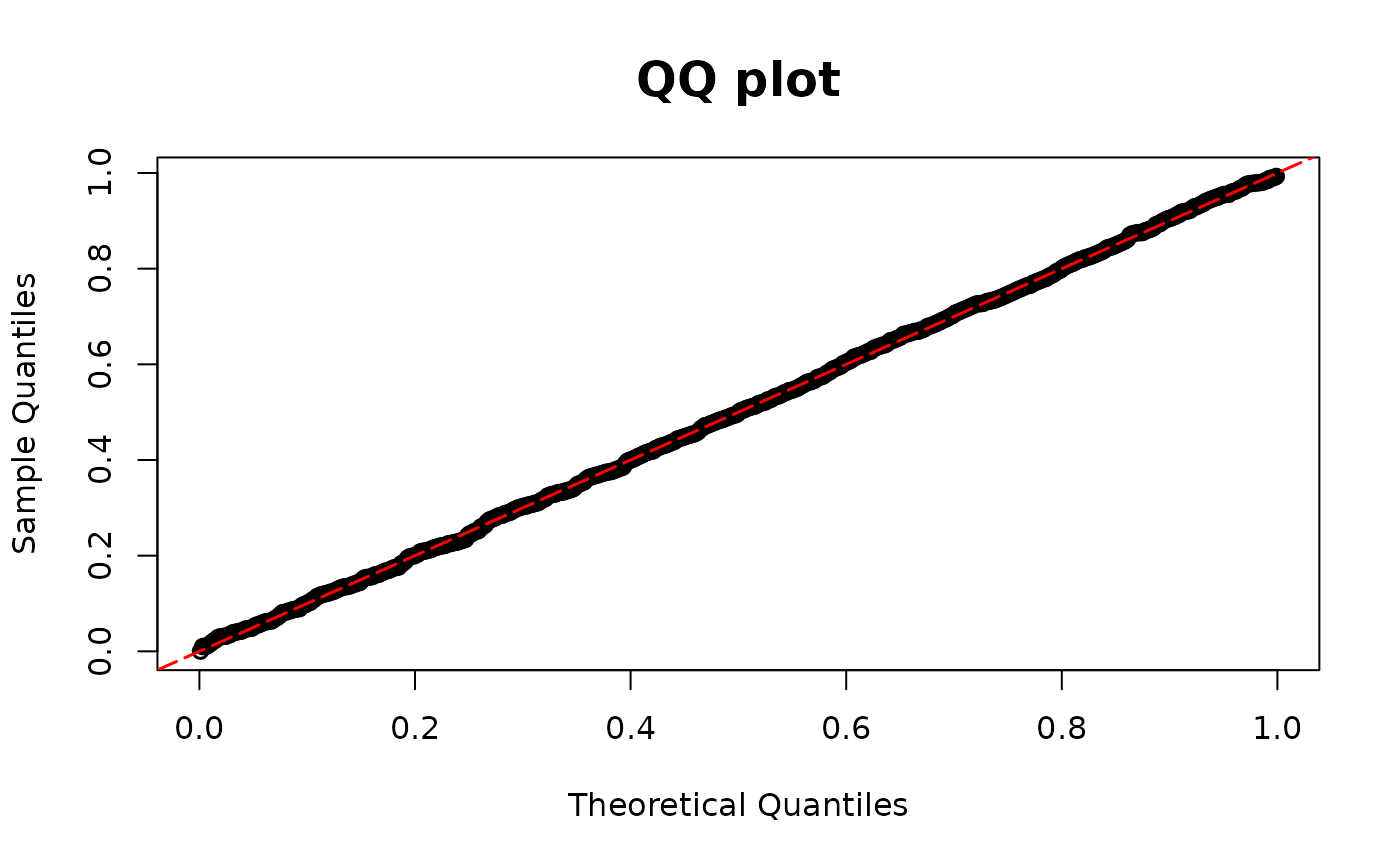
# True model
model1 <- glm.nb(y ~ x1 + x2)
y1 <- model1$y
fitted1 <- fitted(model1)
size1 <- model1$theta
resid.nb1 <- dpit_nb(y=y1, mu=fitted1, size=size1)


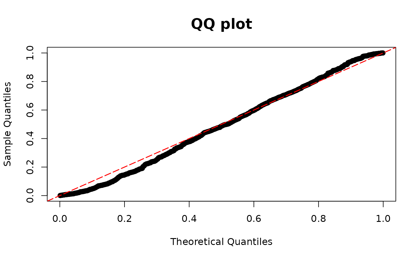
# Overdispersion
model2 <- glm(y ~ x1 + x2, family = poisson(link = "log"))
y2 <- model2$y
fitted2 <- fitted(model2)
resid.nb2 <- dpit_pois(y=y2, mu=fitted2)