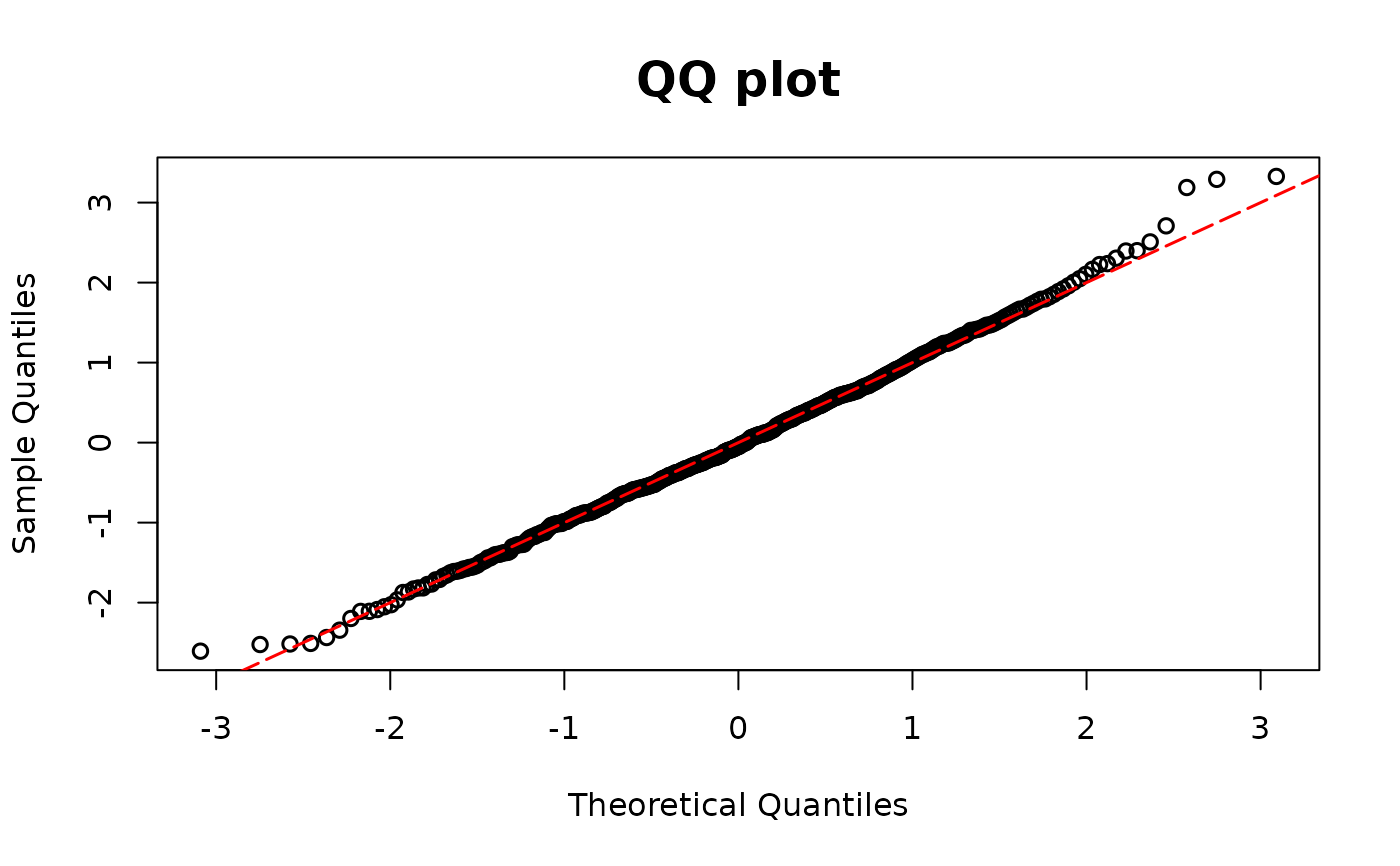
Residuals for regression models with two-part outcomes

Calculates DPIT proposed residuals for model for semi-continuous outcomes. resid_2pm can be used either with model0 and model1 or with part0 and part1 as arguments.

Usage

resid_2pm(model0, model1, y, part0, part1, plot=TRUE, scale = "normal")

Arguments

model0: Model object for 0 outcomes (e.g., logistic regression)
model1: Model object for the continuous part (gamma regression)
y: Semicontinuous outcome variables
part0: Alternative argument to model0. One can supply the sequence of probabilities $P(Y_i=0),~i=1,\ldots,n$.
part1: Alternative argument to model1. One can fit a regression model on the positive data and supply their probability integral transform. Note that the length of part1 is the number of positive values in y and can be shorter than part0.
plot: A logical value indicating whether or not to return QQ-plot
scale: You can choose the scale of the residuals among normal and uniform scales. The default scale is normal.

Value

Residuals. If plot=TRUE, also produces a QQ plot.

Details

The DPIT residuals for regression models with semi-continuous outcomes are $$\hat{r}_i=\frac{\hat{F}(Y_i|\mathbf{X}_i)}{n}\sum_{j=1}^n1\left(\hat{p}_0(\mathbf{X}_j)\leq \hat{F}(Y_i|\mathbf{X}_i)\right), i=1,\ldots,n,$$ where $\hat{p}_0(\mathbf{X}_i)$ is the fitted probability of zero, and $\hat{F}(\cdot|\mathbf{X}_i)$ is the fitted cumulative distribution function for the $i$th observation. Furthermore, $$\hat{F}(y|\mathbf{x})=\hat{p}_0(\mathbf{x})+\left(1-\hat{p}_0(\mathbf{x})\right)\hat{G}(y|\mathbf{x})$$ where $\hat{G}$ is the fitted cumulative distribution for the positive data.

In two-part models, the probability of zero can be modeled using a logistic regression, model0, while the positive observations can be modeled using a gamma regression, model1. Users can choose to use different models and supply the resulting probability transforms. part0 should be the sequence of fitted probabilities of zeros $\hat{p}_0(\mathbf{X}_i) ,~i=1,\ldots,n$. part1 should be the probability integral transform of the positive part $\hat{G}(Y_i|\mathbf{X}_i)$. Note that the length of part1 is the number of positive values in y and can be shorter than part0.

Examples

library(MASS)
n <- 500
beta10 <- 1
beta11 <- -2
beta12 <- -1
beta13 <- -1
beta14 <- -1
beta15 <- -2
x11 <- rnorm(n)
x12 <- rbinom(n, size = 1, prob = 0.4)

p1 <- 1 / (1 + exp(-(beta10 + x11 * beta11 + x12 * beta12)))
lambda1 <- exp(beta13 + beta14 * x11 + beta15 * x12)
y2 <- rgamma(n, scale = lambda1 / 2, shape = 2)
y <- rep(0, n)
u <- runif(n, 0, 1)
ind1 <- which(u >= p1)
y[ind1] <- y2[ind1]

# models as input
mgamma <- glm(y[ind1] ~ x11[ind1] + x12[ind1], family = Gamma(link = "log"))
m10 <- glm(y == 0 ~ x12 + x11, family = binomial(link = "logit"))
resid.model <- resid_2pm(model0 = m10, model1 = mgamma, y = y)

# PIT as input
cdfgamma <- pgamma(y[ind1],
  scale = mgamma$fitted.values * gamma.dispersion(mgamma),
  shape = 1 / gamma.dispersion(mgamma)
)
p1f <- m10$fitted.values
resid.pit <- resid_2pm(y = y, part0 = p1f, part1 = cdfgamma)