Residuals for regression models with ordinal outcomes

Computes DPIT residuals for regression models with ordinal outcomes using observed outcomes (y), ordinal outcome levels (level) and their fitted category probabilities (fitprob).

Usage

dpit_ordi(y, level, fitprob, plot=TRUE, scale="normal", line_args=list(), ...)

Arguments

y: An observed ordinal outcome vector.
level: The names of the response levels. For instance, c(0,1,2).
fitprob: A matrix of fitted category probabilities. Each row corresponds to an observation, and column j contains the fitted probability P(Y_i = j).
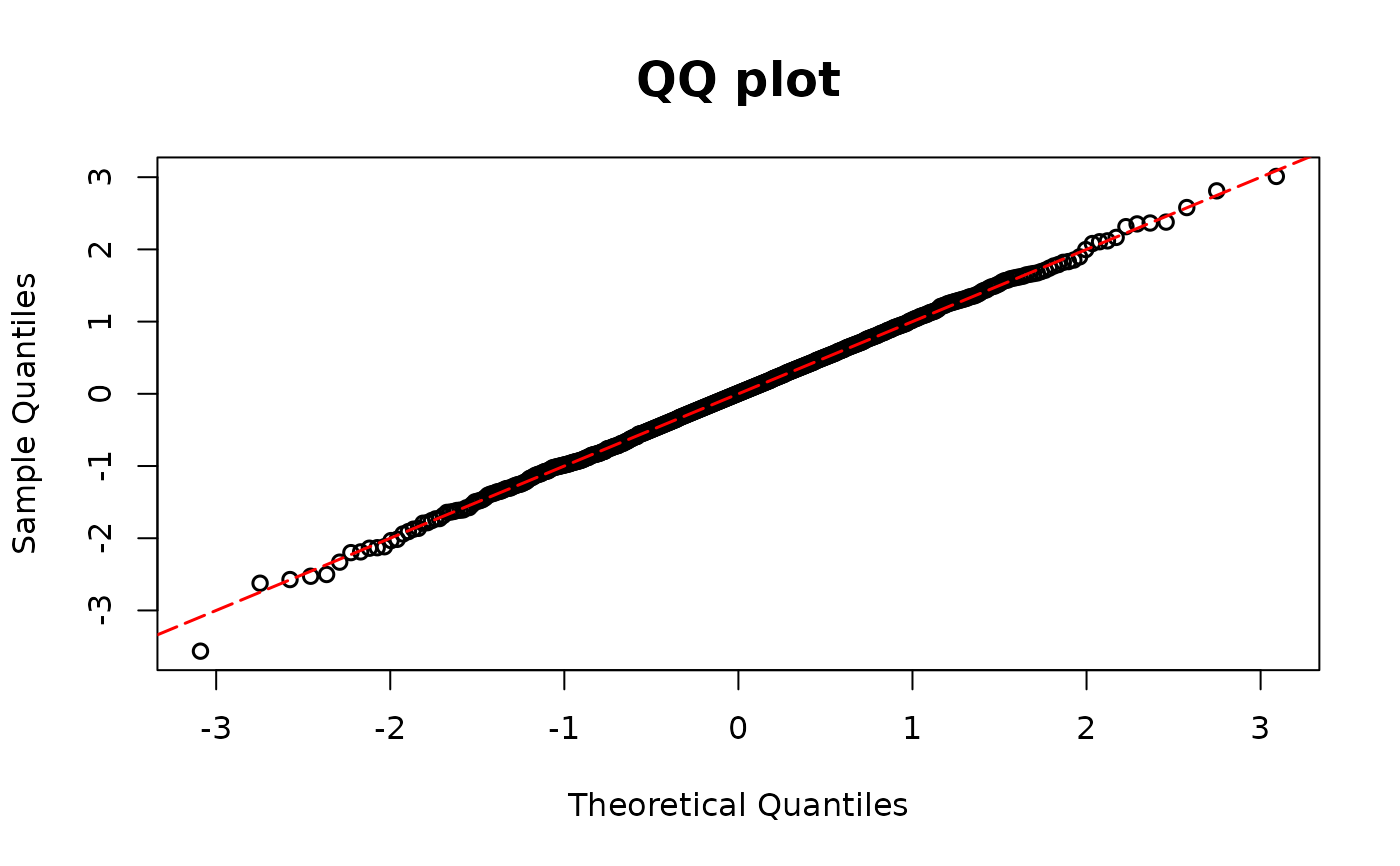
plot: A logical value indicating whether or not to return QQ-plot
scale: You can choose the scale of the residuals among normal and uniform. The sample quantiles of the residuals are plotted against the theoretical quantiles of a standard normal distribution under the normal scale, and against the theoretical quantiles of a uniform (0,1) distribution under the uniform scale. The default scale is normal.
line_args: A named list of graphical parameters passed to graphics::abline() to modify the reference (red) 45° line in the QQ plot. If left empty, a default red dashed line is drawn.
...: Additional graphical arguments passed to stats::qqplot() for customizing the QQ plot (e.g., pch, col, cex, xlab, ylab).

Value

DPIT residuals.

Details

For formulation details on discrete outcomes, see dpit.

Examples

## Ordinal example
library(MASS)
n <- 500
x1 <- rnorm(n, mean = 2)
beta1 <- 3
# True model
p0 <- plogis(1, location = beta1 * x1)
p1 <- plogis(4, location = beta1 * x1) - p0
p2 <- 1 - p0 - p1
genemult <- function(p) {
 rmultinom(1, size = 1, prob = c(p[1], p[2], p[3]))
}
test <- apply(cbind(p0, p1, p2), 1, genemult)
y1 <- rep(0, n)
y1[which(test[1, ] == 1)] <- 0
y1[which(test[2, ] == 1)] <- 1
y1[which(test[3, ] == 1)] <- 2
multimodel <- polr(as.factor(y1) ~ x1, method = "logistic")

y1 <- multimodel$model[,1]
lev1 <- multimodel$lev
fitprob1 <- fitted(multimodel)

resid.ord <- dpit_ordi(y=y1, level=lev1, fitprob=fitprob1)