DPIT residuals for regression models with various non-continuous outcomes
Source:R/dpit_main.R
dpit.RdCalculates DPIT residuals for regression models with non-continuous outcomes.
In particular, model assumptions for GLMs with discrete outcomes (e.g., binary, Poisson, and negative binomial), ordinal
regression models, zero-inflated regression models, and semicontinuous outcome
models can be assessed using dpit().
Usage
dpit(model, plot=TRUE, scale="normal", line_args=list(), ...)Arguments
- model
A model object.
- plot
A logical value indicating whether or not to return QQ-plot
- scale
You can choose the scale of the residuals among
normalanduniform. The sample quantiles of the residuals are plotted against the theoretical quantiles of a standard normal distribution under the normal scale, and against the theoretical quantiles of a uniform (0,1) distribution under the uniform scale. The default scale isnormal.- line_args
A named list of graphical parameters passed to
graphics::abline()to modify the reference (red) 45° line in the QQ plot. If left empty, a default red dashed line is drawn.- ...
Additional graphical arguments passed to
stats::qqplot()for customizing the QQ plot (e.g.,pch,col,cex,xlab,ylab).
Details
This function determines the appropriate computation based on the class of
model. The supported model objects and outcome types are listed below.
In addition to the class-based interface, the package also provides
distribution-specific DPIT calculators. If a fitted model comes from a
different class but has a supported outcome distribution, users can call
the corresponding distribution-based function directly.
For instance, for a regression model with Poisson outcomes,
one can use dpit to calculate the residuals if
the model is fit using glm function, or to use dpit_pois upon supplying fitted mean values.
Discrete outcomes
Zero-inflated discrete outcomes
zeroinflwithdist = "poisson"(seedpit_zpois).
Semicontinuous outcomes
Tobit regression via
tobitfromAERorvglmfromVGAM(seedpit_tobit).Tweedie regression via
glmwith a Tweedie family (seedpit_tweedie).
Formulation for Discrete and Zero-Inflated Outcomes:
The DPIT residual for the \(i\)th observation is defined as follows:
$$\hat{r}(Y_i|X_i) = \hat{G}\bigg(\hat{F}(Y_i|\mathbf{X}_i)\bigg)$$
where
$$\hat{G}(s) = \frac{1}{n-1}\sum_{j=1, j \neq i}^{n}\hat{F}\bigg(\hat{F}^{(-1)}(\mathbf{X}_j)\bigg|\mathbf{X}_j\bigg)$$
and \(\hat{F}\) refers to the fitted cumulative distribution function.
When scale="uniform", DPIT residuals should closely follow a uniform distribution, otherwise it implies model deficiency.
When scale="normal", it applies the normal quantile transformation to the DPIT residuals
$$\Phi^{-1}\left[\hat{r}(Y_i|\mathbf{X}_i)\right],i=1,\ldots,n.$$ The null pattern is the standard normal distribution in this case.
Formulation for Semicontinuous Outcomes:
The DPIT residuals for regression models with semi-continuous outcomes are $$\hat{r}_i=\frac{\hat{F}(Y_i|\mathbf{X}_i)}{n}\sum_{j=1}^n1\left(\hat{p}_0(\mathbf{X}_j)\leq \hat{F}(Y_i|\mathbf{X}_i)\right), i=1,\ldots,n,$$
where \(\hat{p}_0(\mathbf{X}_i)\) is the fitted probability of zero, and \(\hat{F}(\cdot|\mathbf{X}_i)\) is the fitted cumulative distribution function for the \(i\)th observation. Furthermore, $$\hat{F}(y|\mathbf{x})=\hat{p}_0(\mathbf{x})+\left(1-\hat{p}_0(\mathbf{x})\right)\hat{G}(y|\mathbf{x})$$
where \(\hat{G}\) is the fitted cumulative distribution for the positive data.
References
L. Yang. Double probability integral transform residuals for regression models with discrete outcomes. Journal of Computational and Graphical Statistics, 33(3), pp.787–803, 2024.
L. Yang. Diagnostics for regression models with semicontinuous outcomes. Biometrics, 80(1), ujae007, 2024.
Examples
library(MASS)
n <- 500
set.seed(1234)
## Negative Binomial example
# Covariates
x1 <- rnorm(n)
x2 <- rbinom(n, 1, 0.7)
### Parameters
beta0 <- -2
beta1 <- 2
beta2 <- 1
size1 <- 2
lambda1 <- exp(beta0 + beta1 * x1 + beta2 * x2)
# generate outcomes
y <- rnbinom(n, mu = lambda1, size = size1)
# True model
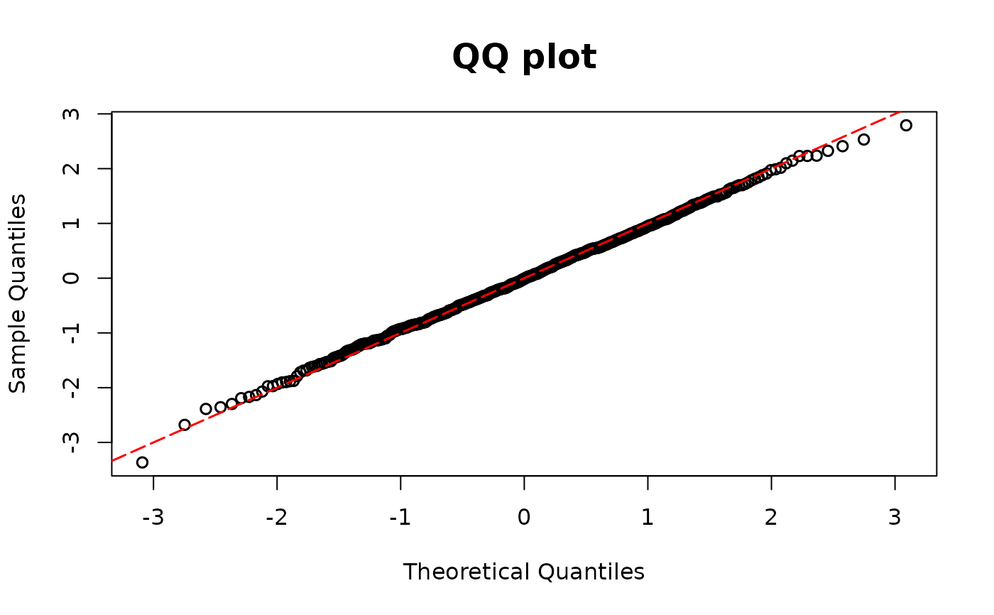
model1 <- glm.nb(y ~ x1 + x2)
resid.nb1 <- dpit(model1, plot = TRUE, scale = "uniform")
 # Overdispersion
model2 <- glm(y ~ x1 + x2, family = poisson(link = "log"))
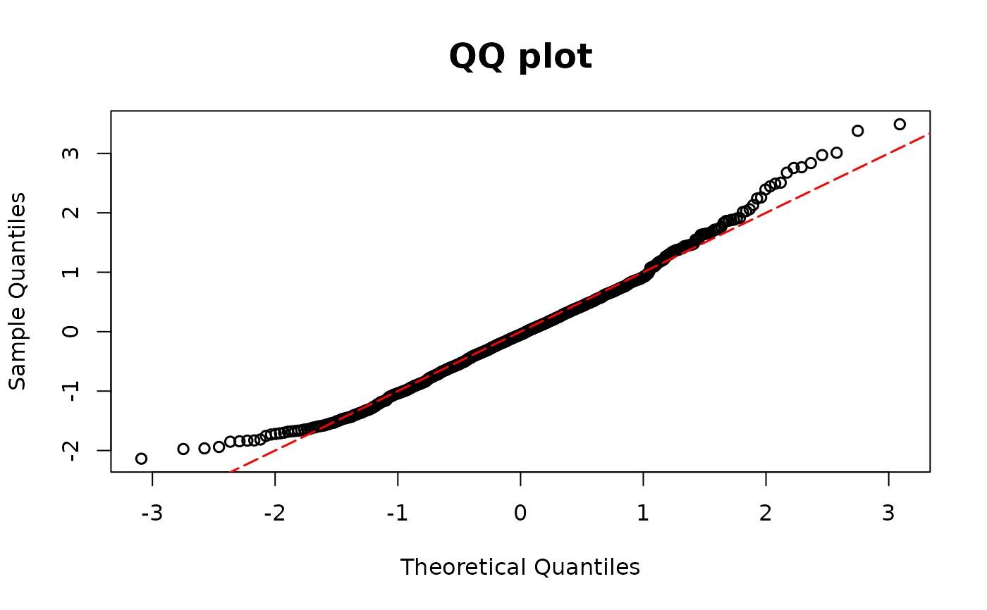
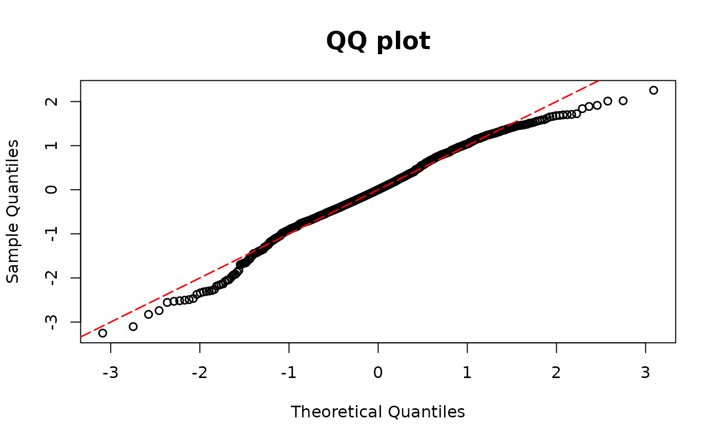
resid.nb2 <- dpit(model2, plot = TRUE, scale = "normal")
# Overdispersion
model2 <- glm(y ~ x1 + x2, family = poisson(link = "log"))
resid.nb2 <- dpit(model2, plot = TRUE, scale = "normal")
 ## Binary example
n <- 500
set.seed(1234)
# Covariates
x1 <- rnorm(n, 1, 1)
x2 <- rbinom(n, 1, 0.7)
# Coefficients
beta0 <- -5
beta1 <- 2
beta2 <- 1
beta3 <- 3
q1 <- 1 / (1 + exp(beta0 + beta1 * x1 + beta2 * x2 + beta3 * x1 * x2))
y1 <- rbinom(n, size = 1, prob = 1 - q1)
# True model
model01 <- glm(y1 ~ x1 * x2, family = binomial(link = "logit"))
resid.bin1 <- dpit(model01, plot = TRUE)
## Binary example
n <- 500
set.seed(1234)
# Covariates
x1 <- rnorm(n, 1, 1)
x2 <- rbinom(n, 1, 0.7)
# Coefficients
beta0 <- -5
beta1 <- 2
beta2 <- 1
beta3 <- 3
q1 <- 1 / (1 + exp(beta0 + beta1 * x1 + beta2 * x2 + beta3 * x1 * x2))
y1 <- rbinom(n, size = 1, prob = 1 - q1)
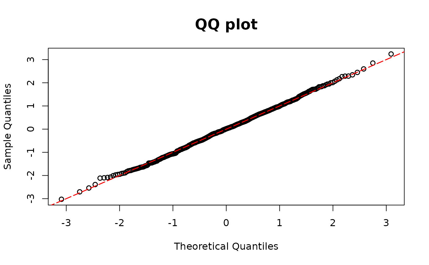
# True model
model01 <- glm(y1 ~ x1 * x2, family = binomial(link = "logit"))
resid.bin1 <- dpit(model01, plot = TRUE)
 # Missing covariates
model02 <- glm(y1 ~ x1, family = binomial(link = "logit"))
resid.bin2 <- dpit(model02, plot = TRUE)
# Missing covariates
model02 <- glm(y1 ~ x1, family = binomial(link = "logit"))
resid.bin2 <- dpit(model02, plot = TRUE)
 ## Poisson example
n <- 500
set.seed(1234)
# Covariates
x1 <- rnorm(n)
x2 <- rbinom(n, 1, 0.7)
# Coefficients
beta0 <- -2
beta1 <- 2
beta2 <- 1
lambda1 <- exp(beta0 + beta1 * x1 + beta2 * x2)
y <- rpois(n, lambda1)
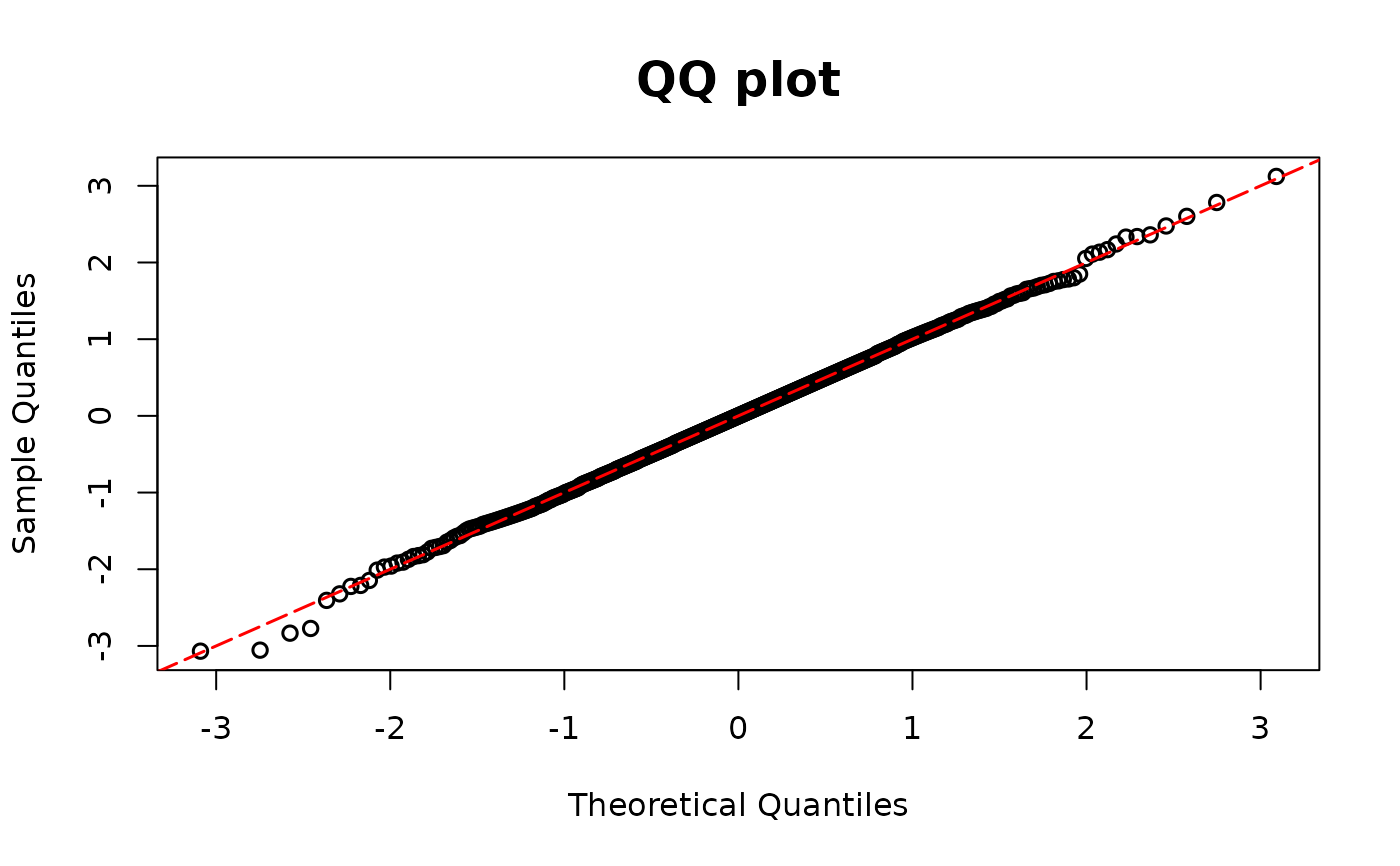
# True model
poismodel1 <- glm(y ~ x1 + x2, family = poisson(link = "log"))
resid.poi1 <- dpit(poismodel1, plot = TRUE)
## Poisson example
n <- 500
set.seed(1234)
# Covariates
x1 <- rnorm(n)
x2 <- rbinom(n, 1, 0.7)
# Coefficients
beta0 <- -2
beta1 <- 2
beta2 <- 1
lambda1 <- exp(beta0 + beta1 * x1 + beta2 * x2)
y <- rpois(n, lambda1)
# True model
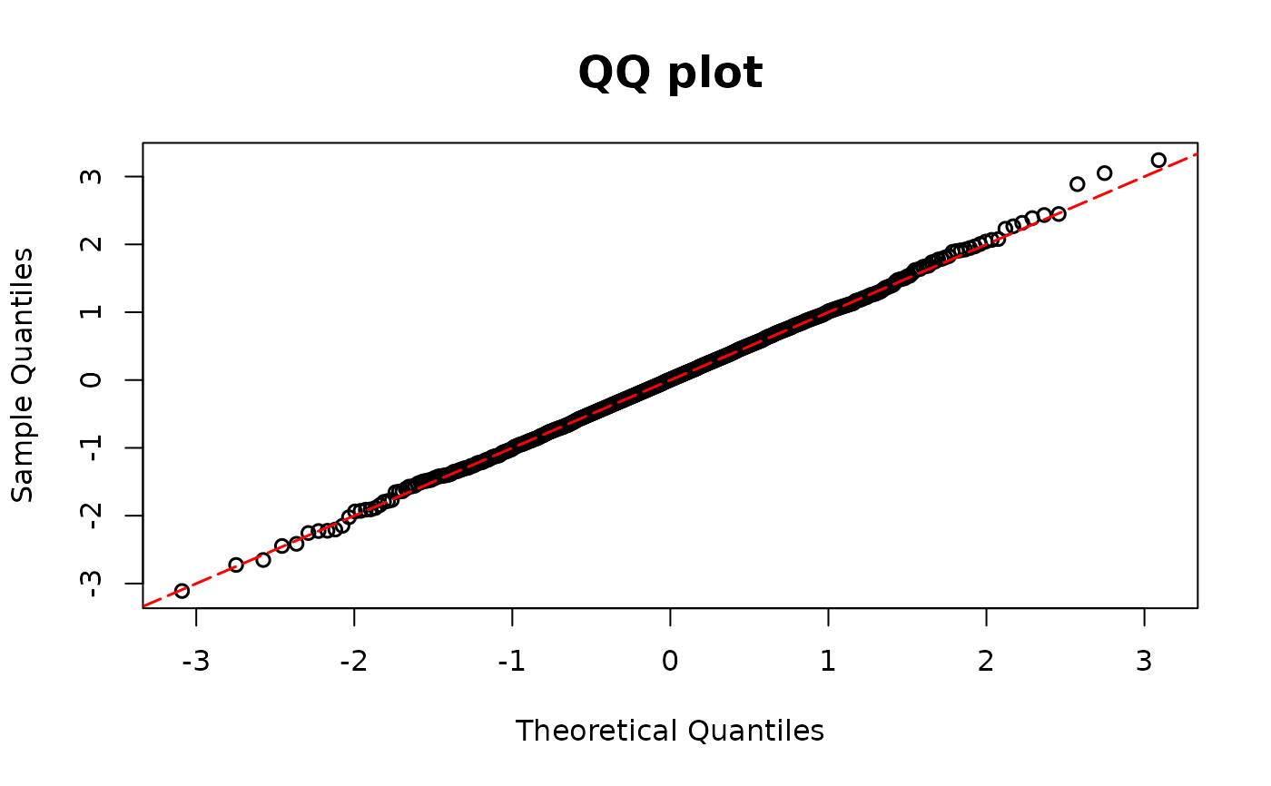
poismodel1 <- glm(y ~ x1 + x2, family = poisson(link = "log"))
resid.poi1 <- dpit(poismodel1, plot = TRUE)
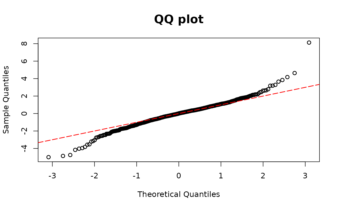
 # Enlarge three outcomes
y <- rpois(n, lambda1) + c(rep(0, (n - 3)), c(10, 15, 20))
poismodel2 <- glm(y ~ x1 + x2, family = poisson(link = "log"))
resid.poi2 <- dpit(poismodel2, plot = TRUE)
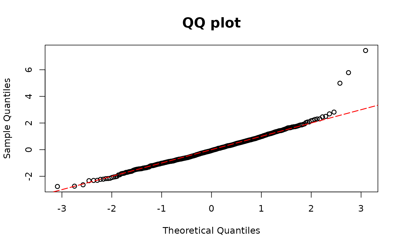
# Enlarge three outcomes
y <- rpois(n, lambda1) + c(rep(0, (n - 3)), c(10, 15, 20))
poismodel2 <- glm(y ~ x1 + x2, family = poisson(link = "log"))
resid.poi2 <- dpit(poismodel2, plot = TRUE)
 ## Ordinal example
n <- 500
set.seed(1234)
# Covariates
x1 <- rnorm(n, mean = 2)
# Coefficient
beta1 <- 3
# True model
p0 <- plogis(1, location = beta1 * x1)
p1 <- plogis(4, location = beta1 * x1) - p0
p2 <- 1 - p0 - p1
genemult <- function(p) {
rmultinom(1, size = 1, prob = c(p[1], p[2], p[3]))
}
test <- apply(cbind(p0, p1, p2), 1, genemult)
y1 <- rep(0, n)
y1[which(test[1, ] == 1)] <- 0
y1[which(test[2, ] == 1)] <- 1
y1[which(test[3, ] == 1)] <- 2
multimodel <- polr(as.factor(y1) ~ x1, method = "logistic")
resid.ord1 <- dpit(multimodel, plot = TRUE)
## Ordinal example
n <- 500
set.seed(1234)
# Covariates
x1 <- rnorm(n, mean = 2)
# Coefficient
beta1 <- 3
# True model
p0 <- plogis(1, location = beta1 * x1)
p1 <- plogis(4, location = beta1 * x1) - p0
p2 <- 1 - p0 - p1
genemult <- function(p) {
rmultinom(1, size = 1, prob = c(p[1], p[2], p[3]))
}
test <- apply(cbind(p0, p1, p2), 1, genemult)
y1 <- rep(0, n)
y1[which(test[1, ] == 1)] <- 0
y1[which(test[2, ] == 1)] <- 1
y1[which(test[3, ] == 1)] <- 2
multimodel <- polr(as.factor(y1) ~ x1, method = "logistic")
resid.ord1 <- dpit(multimodel, plot = TRUE)
 ## Non-Proportionality
n <- 500
set.seed(1234)
x1 <- rnorm(n, mean = 2)
beta1 <- 3
beta2 <- 1
p0 <- plogis(1, location = beta1 * x1)
p1 <- plogis(4, location = beta2 * x1) - p0
p2 <- 1 - p0 - p1
genemult <- function(p) {
rmultinom(1, size = 1, prob = c(p[1], p[2], p[3]))
}
test <- apply(cbind(p0, p1, p2), 1, genemult)
y1 <- rep(0, n)
y1[which(test[1, ] == 1)] <- 0
y1[which(test[2, ] == 1)] <- 1
y1[which(test[3, ] == 1)] <- 2
multimodel <- polr(as.factor(y1) ~ x1, method = "logistic")
resid.ord2 <- dpit(multimodel, plot = TRUE)
## Non-Proportionality
n <- 500
set.seed(1234)
x1 <- rnorm(n, mean = 2)
beta1 <- 3
beta2 <- 1
p0 <- plogis(1, location = beta1 * x1)
p1 <- plogis(4, location = beta2 * x1) - p0
p2 <- 1 - p0 - p1
genemult <- function(p) {
rmultinom(1, size = 1, prob = c(p[1], p[2], p[3]))
}
test <- apply(cbind(p0, p1, p2), 1, genemult)
y1 <- rep(0, n)
y1[which(test[1, ] == 1)] <- 0
y1[which(test[2, ] == 1)] <- 1
y1[which(test[3, ] == 1)] <- 2
multimodel <- polr(as.factor(y1) ~ x1, method = "logistic")
resid.ord2 <- dpit(multimodel, plot = TRUE)