Residuals for regression models with zero-inflated negative binomial outcomes

Computes DPIT residuals for regression models with zero-inflated negative binomial outcomes using the observed counts (y) and their fitted distributional parameters (mu, pzero, size).

Usage

dpit_znb(y, mu, pzero, size, plot=TRUE, scale="normal", line_args=list(), ...)

Arguments

y: An observed outcome vector.
mu: A vector of fitted mean values for the count (non-zero) component.
pzero: A vector of fitted probabilities for the zero-inflation component.
size: A dispersion parameter of the negative binomial distribution.
plot: A logical value indicating whether or not to return QQ-plot
scale: You can choose the scale of the residuals among normal and uniform. The sample quantiles of the residuals are plotted against the theoretical quantiles of a standard normal distribution under the normal scale, and against the theoretical quantiles of a uniform (0,1) distribution under the uniform scale. The default scale is normal.
line_args: A named list of graphical parameters passed to graphics::abline() to modify the reference (red) 45° line in the QQ plot. If left empty, a default red dashed line is drawn.
...: Additional graphical arguments passed to stats::qqplot() for customizing the QQ plot (e.g., pch, col, cex, xlab, ylab).

Value

DPIT residuals.

Details

For formulation details on discrete outcomes, see dpit.

Examples

## Zero-Inflated Negative Binomial
library(pscl)
#> Classes and Methods for R originally developed in the
#> Political Science Computational Laboratory
#> Department of Political Science
#> Stanford University (2002-2015),
#> by and under the direction of Simon Jackman.
#> hurdle and zeroinfl functions by Achim Zeileis.
n <- 500
set.seed(1234)

# Covariates
x1 <- rnorm(n)
x2 <- rbinom(n, 1, 0.7)

# Coefficients
beta0 <- -2
beta1 <-  2
beta2 <-  1
beta00 <- -2
beta10 <-  2

# NB dispersion (size = theta; larger => closer to Poisson)
theta_true <- 1.2

# Mean of NB count part
mu_true <- exp(beta0 + beta1 * x1 + beta2 * x2)

# Excess zero probability (logit)
p0 <- 1 / (1 + exp(-(beta00 + beta10 * x1)))

## simulate outcomes
z  <- rbinom(n, size = 1, prob = 1 - p0)              # 1 => from NB, 0 => structural zero
y1 <- rnbinom(n, size = theta_true, mu = mu_true)     # NB count draw
y  <- ifelse(z == 0, 0, y1)

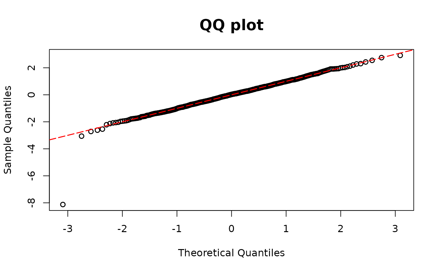
## True model
modelzero1 <- zeroinfl(y ~ x1 + x2 | x1, dist = "negbin", link = "logit")
y1 <- modelzero1$y
mu1    <- stats::predict(modelzero1, type = "count")
pzero1 <- stats::predict(modelzero1, type = "zero")
theta1 <- modelzero1$theta
resid.zero1 <- dpit_znb(y = y1, pzero = pzero1, mu = mu1, size = theta1)


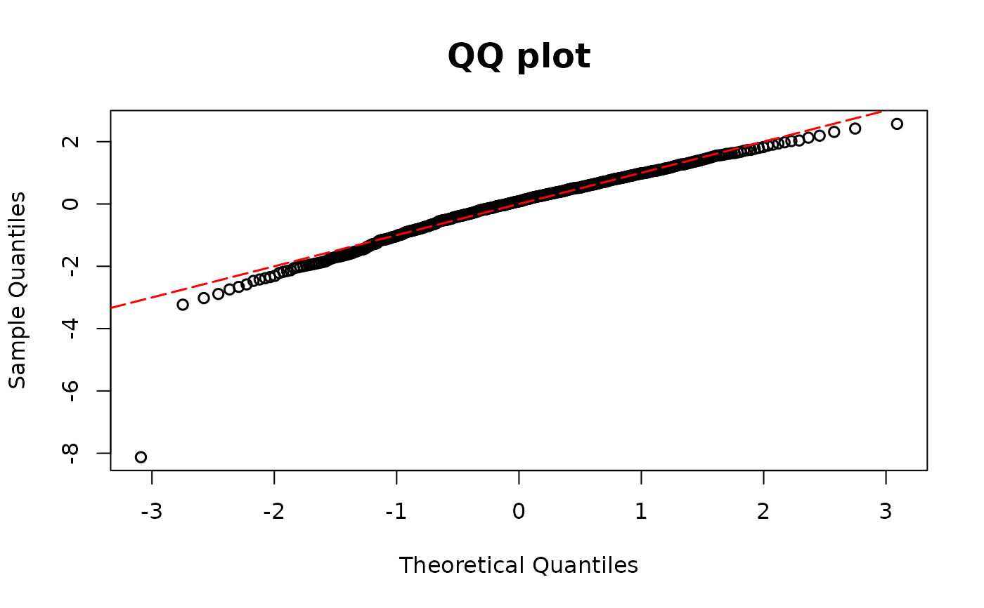
## Ignoring zero-inflation: NB only
modelzero2 <- MASS::glm.nb(y ~ x1 + x2)
y2 <- modelzero2$y
mu2    <- fitted(modelzero2)
theta2 <- modelzero2$theta
resid.zero2 <- dpit_nb(y = y2, mu = mu2, size = theta2)